Working with multiple data sources

With the introduction of v1.5.0 version of Visplore, it is now possible to merge data from different sources directly within Visplore. This guide aims to introduce the fundamental workflows when working with such data.

Importing the first data source (Power Data)

To follow this step-by-step guide, you can use the data files shipped with Visplore. The aim of the analysis is to correlate power and weather data which are stored as different files in addition to comparing different timespans.

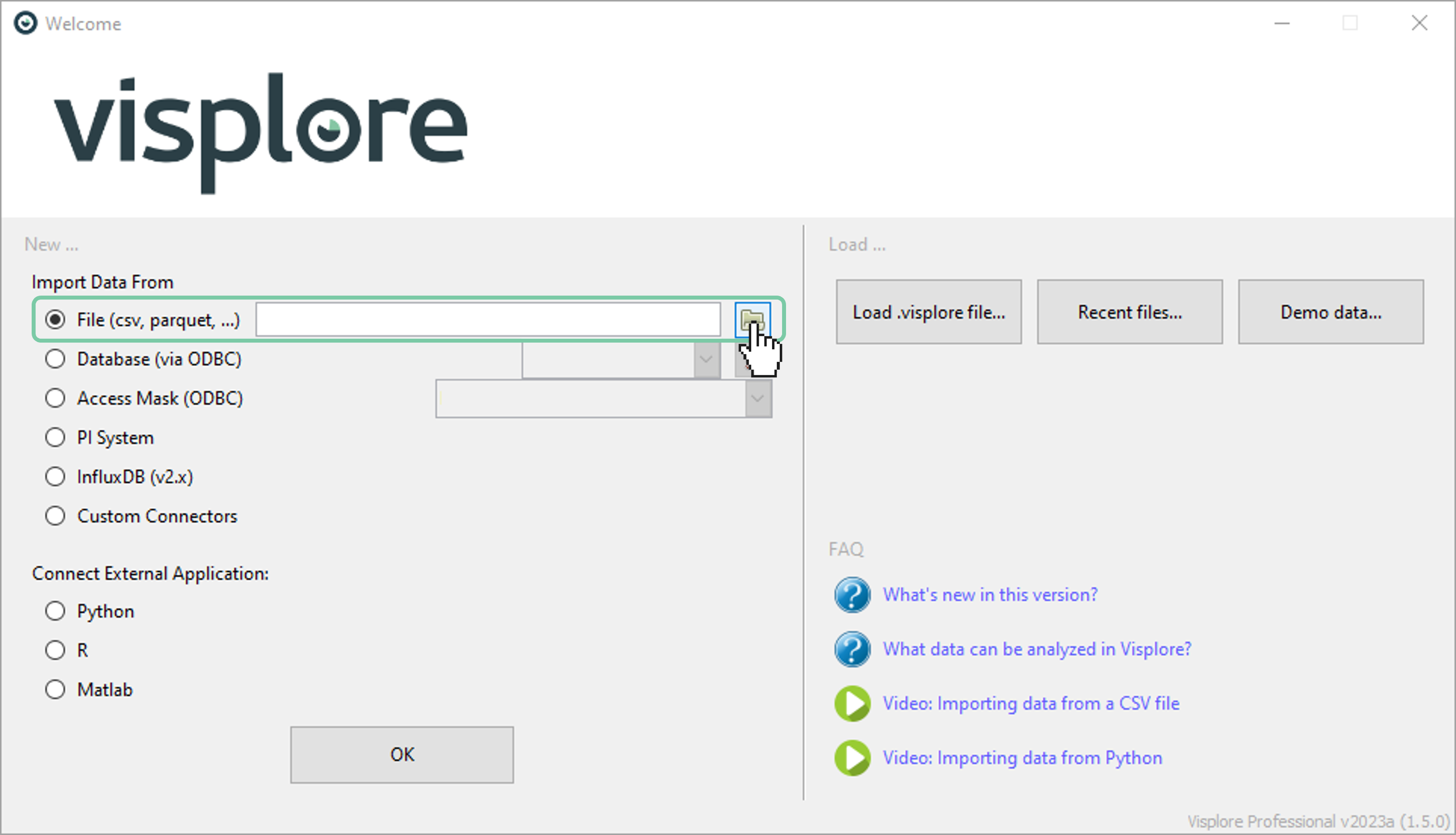
In the welcome dialog, select “File (csv, parquet, …)” and then click the file explorer icon to locate the files.

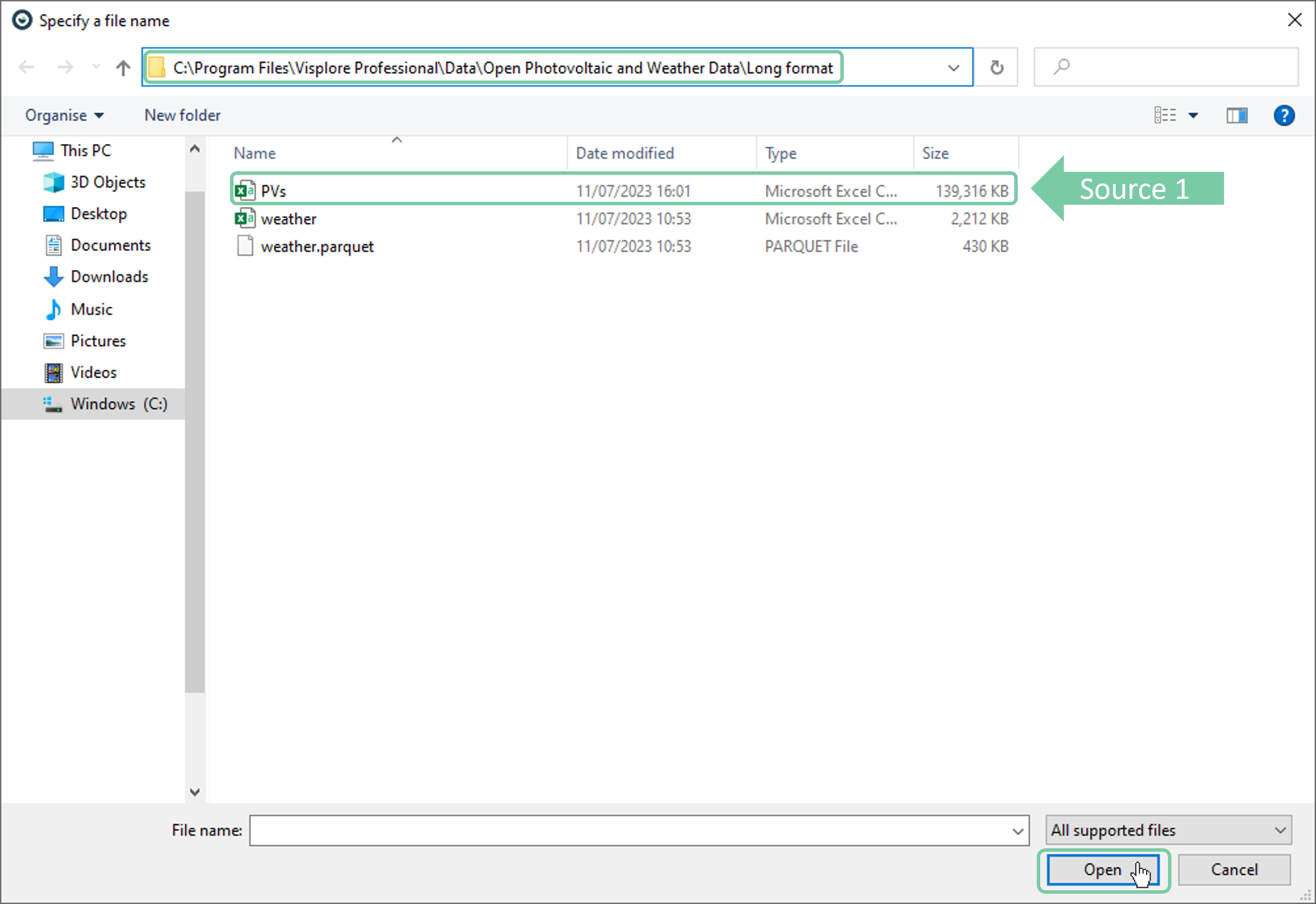
In the file explorer, navigate to the folder where Visplore is installed. Then, locate and select the .csv file named “PVs”. Have a look at the address bar in the image below for help. Click ‘Open’.

Click ‘OK’ in the welcome dialog to start the import.

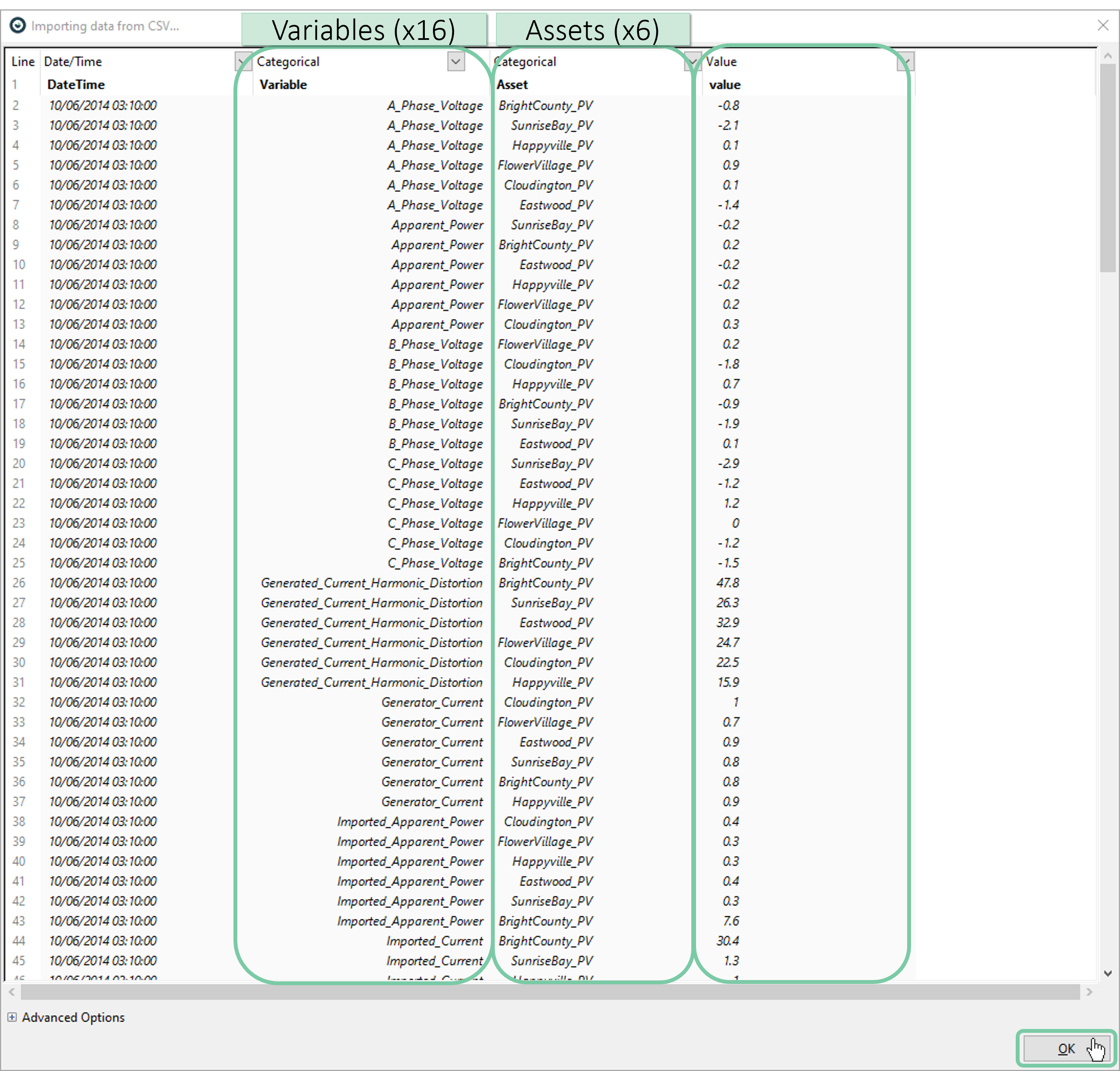
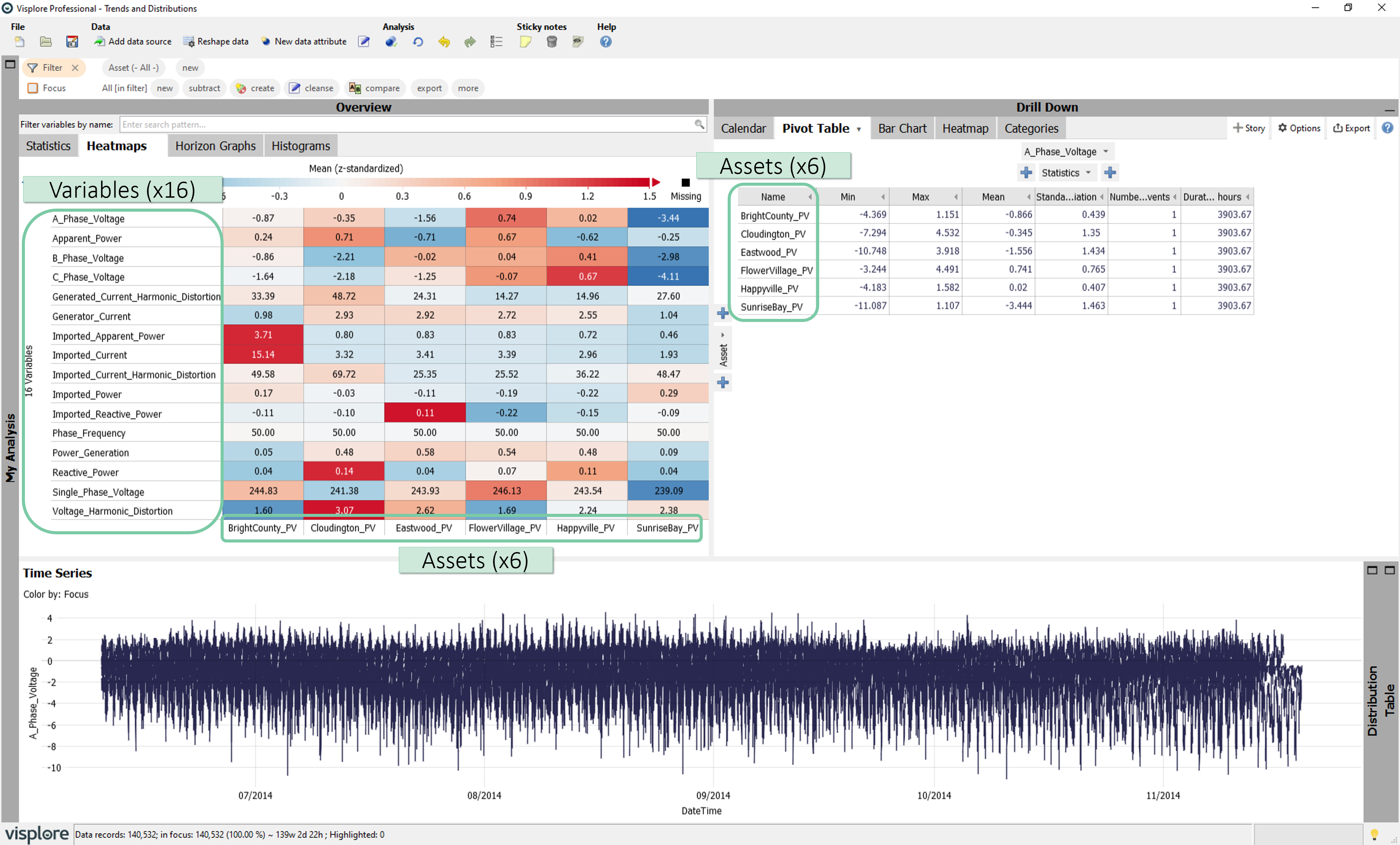
Next, a preview of the data will be shown. This dataset holds 16 variables (sensor measurements) across 6 different assets (photovoltaic power plants) situated nearby. Please notice that the data is in long format i.e., every row of record holds a single value for a single type of measurement (variable) from a single asset. Therefore, there are 96 rows (16x6) per timestamp. Click ‘OK’.

You will notice that Asset/Variable structure definition window will be shown with automatically detected asset and variable suggestions. In general, we would like to accept this suggestion, but for the sake of this guide, uncheck both boxes and click ‘OK’.

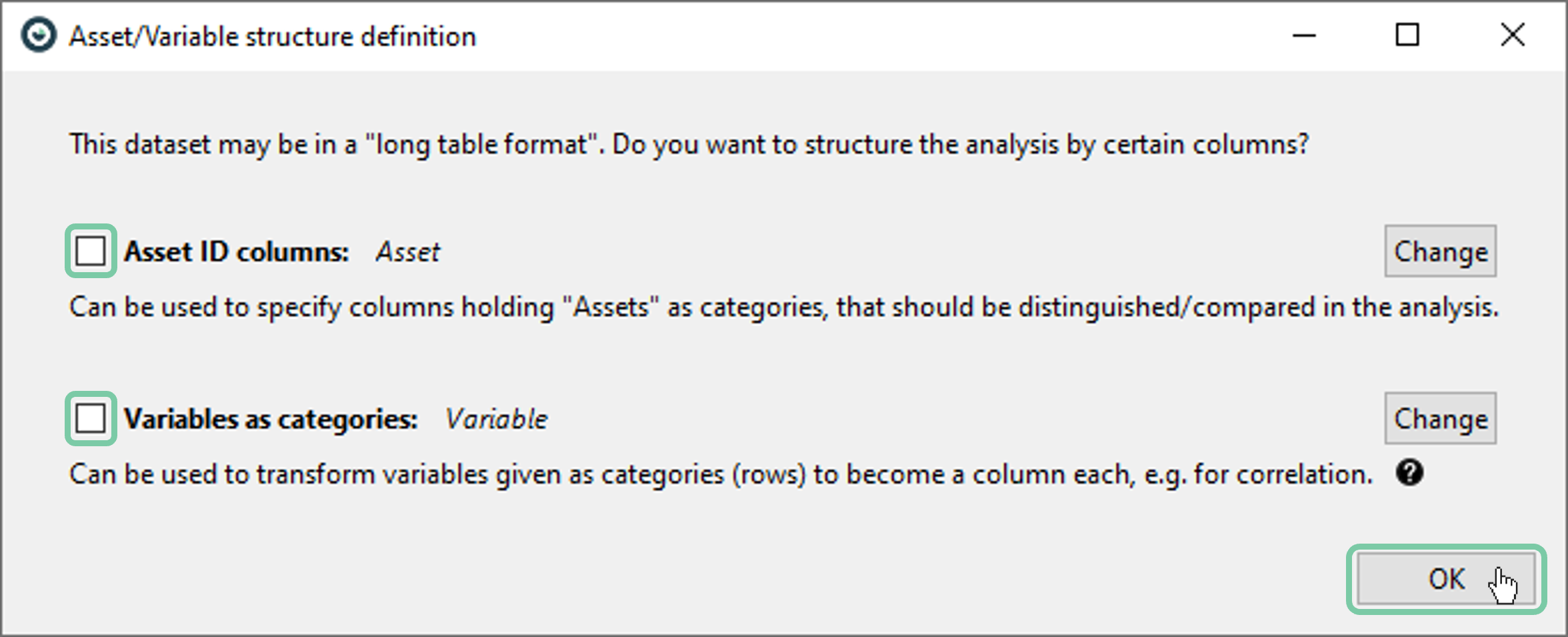
A warning dialog that states the data is quite large and asking if you would like to transform/rasterize it will appear. Just click ‘No’ as we will rasterize the data after importing the second data source anyway.

Transforming the first data source (Power Data) from long format to wide format

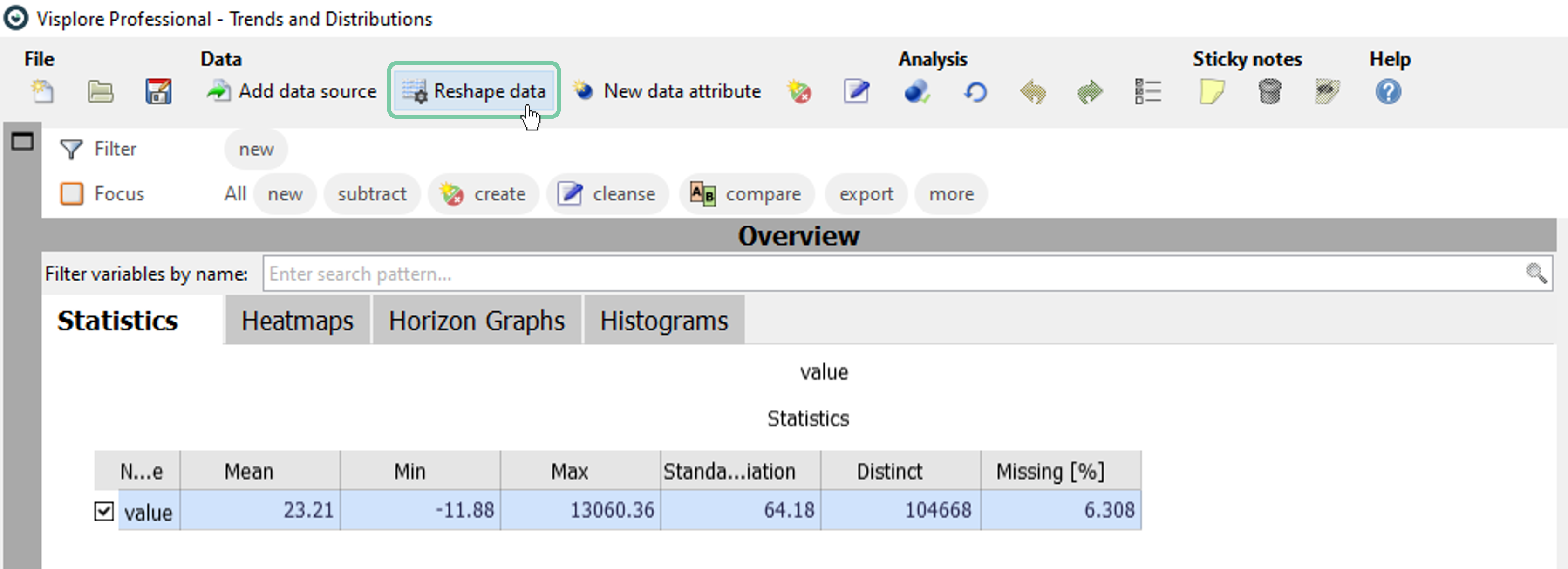
At this point you should see a single variable named ‘value’ that holds more than 2.2 million data records. Due to long format, it is not possible to use this data structure as is, especially for correlation analysis. We would like to transform rows to columns so that the data structure becomes wider, and each distinct variable becomes a unique column.

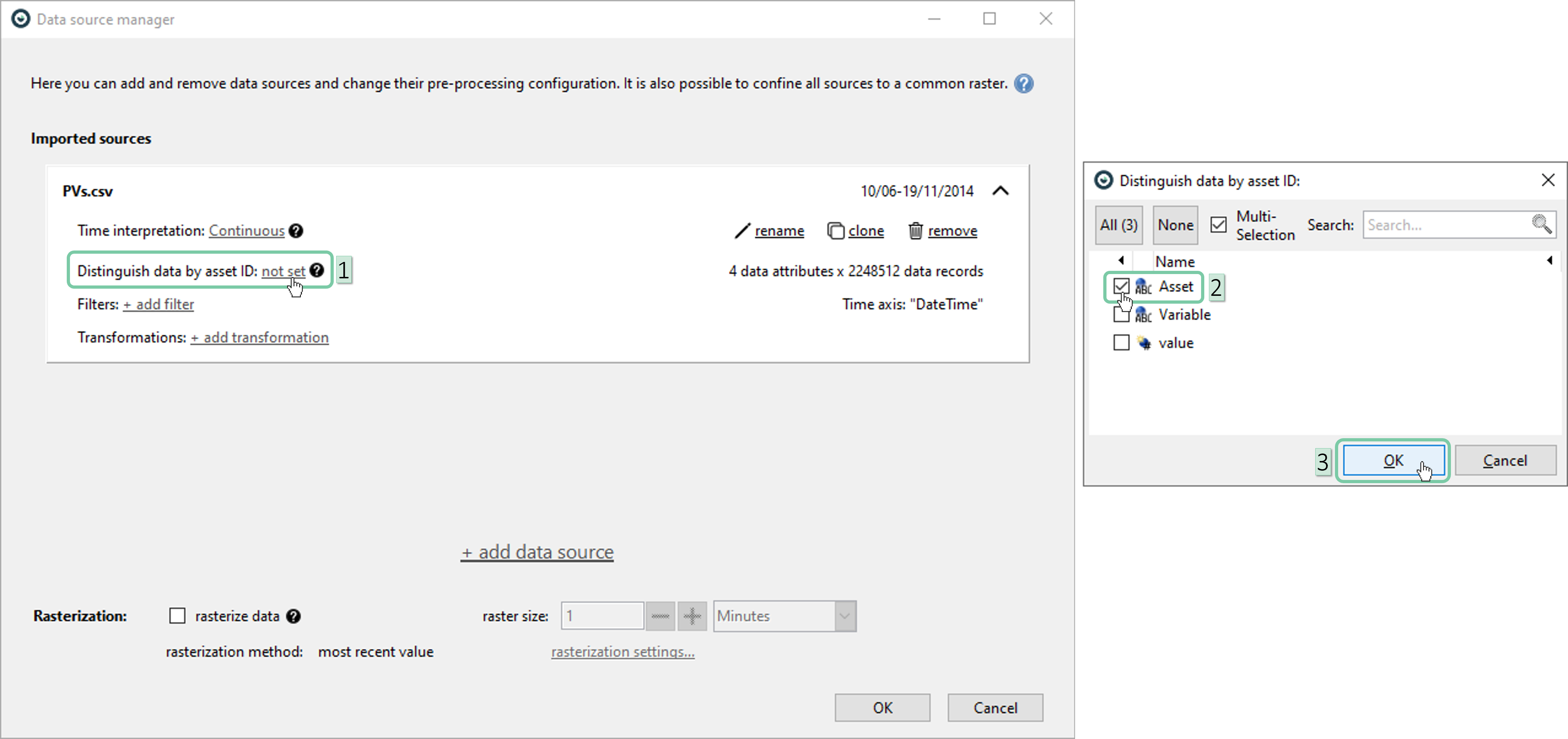
First, we need to set the asset ID to distinguish between 6 different assets. Click on ‘Distinguish data by asset ID’ and select ‘Asset’ in the newly-appeared window. Then click ‘OK’.

Second, click the ‘add transformation’ button and select ‘Rows to columns transformation’. Set the ‘Variable’ as the category column and click ‘OK’. Please make sure that the rest of the transformation dialog is as shown in boxes 5 and 6. Finally, click ‘OK’ two more times in sequence.

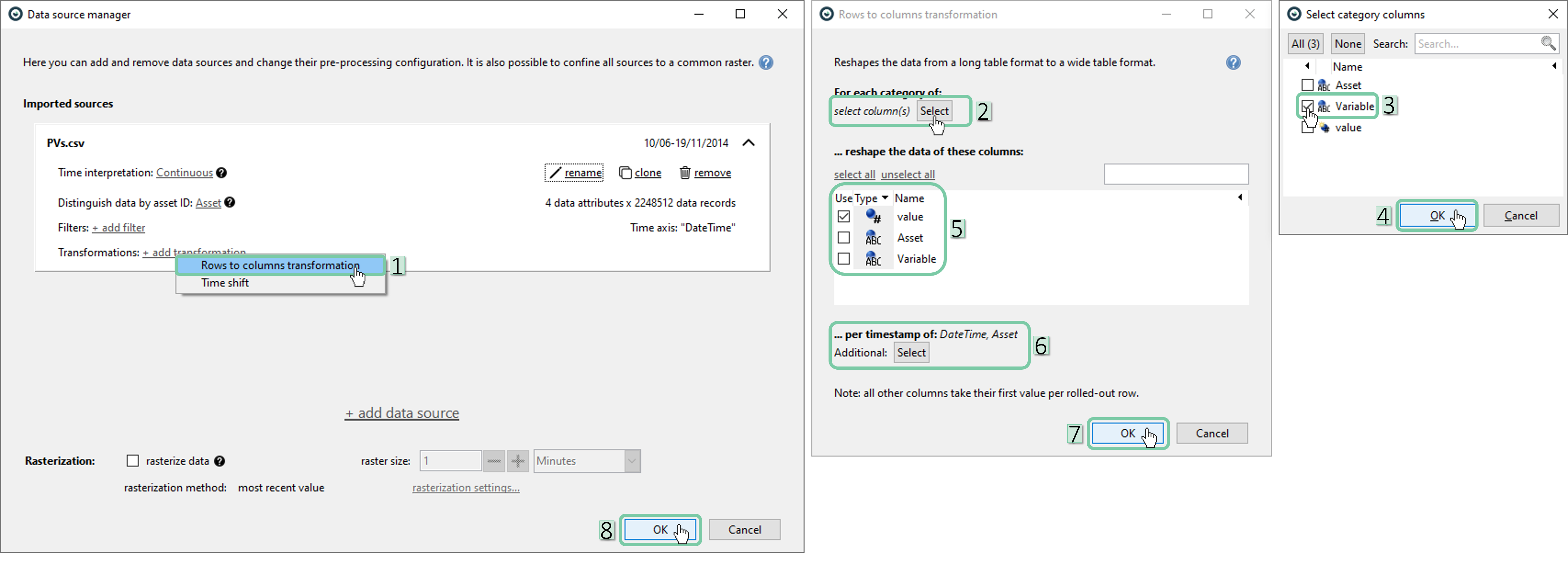
Now, you should notice that the 16 variables that used to be represented as a single column, have become individual data attributes (variables) and number of data records are reduced to 1/16 of its original value. Also notice that asset ID is automatically utilized for distinguishing between assets.

Merging the second data source (Weather Data) into the analysis

Now, as we shaped the first data source to our need, is time to import the second data source and merge both data sources into a single data structure. Before doing so, please notice that the current data source (PVs) have a 10-minute regular interval between consecutive data records.

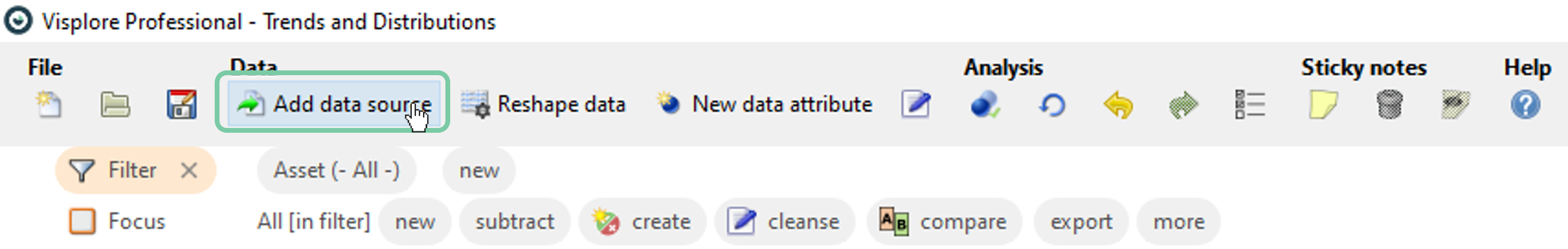
Click ‘Add data source’ from the data toolbar.

In the welcome dialog, select “File (csv, parquet, …)” and then click the file explorer icon to locate the files.

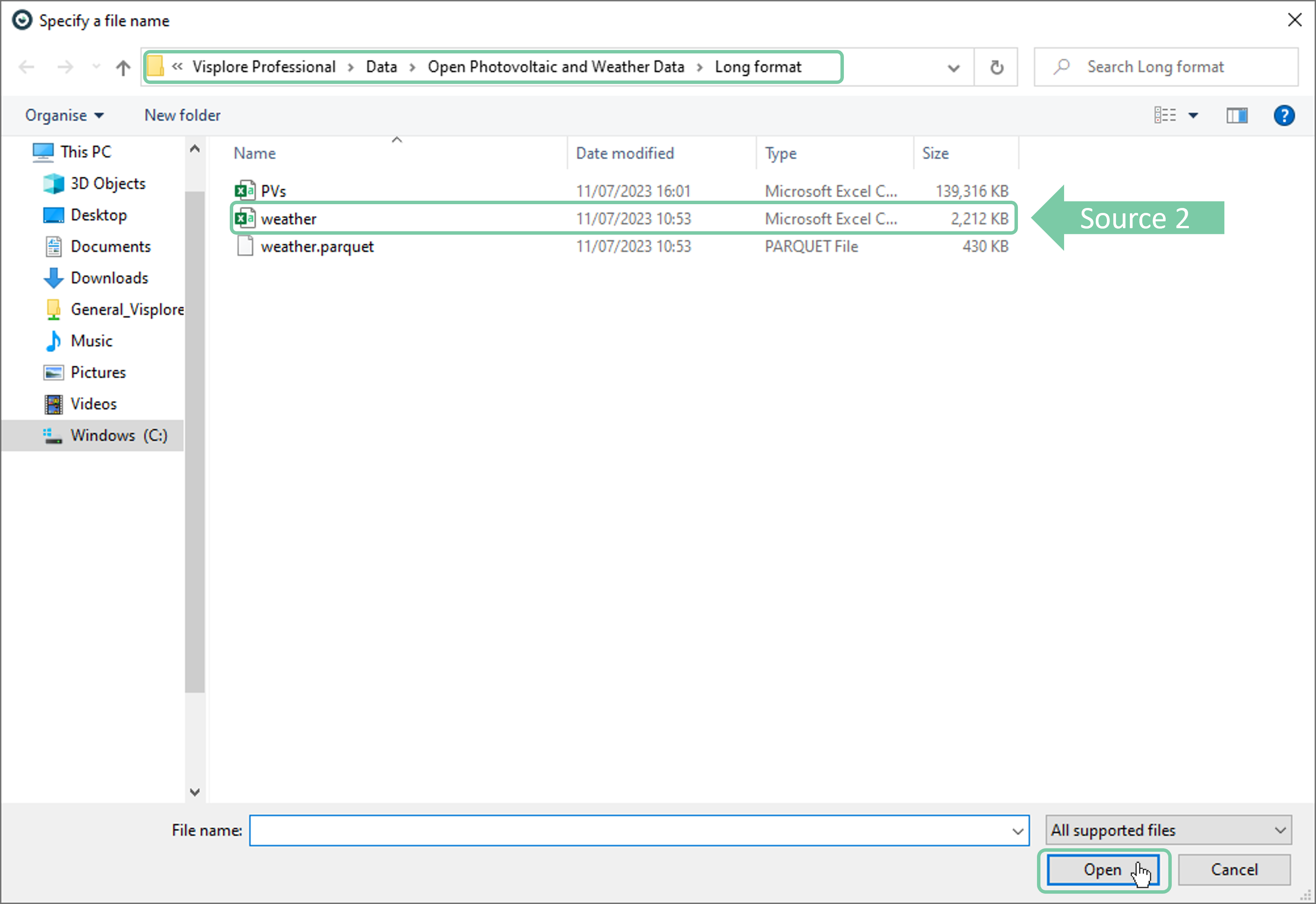
In the file explorer, navigate to the folder where Visplore is installed. Then, locate and select the .csv file named “weather”. Have a look at the address bar in the image below for help. Click ‘Open’.

Click ‘OK’ in the import dialog to start the import.

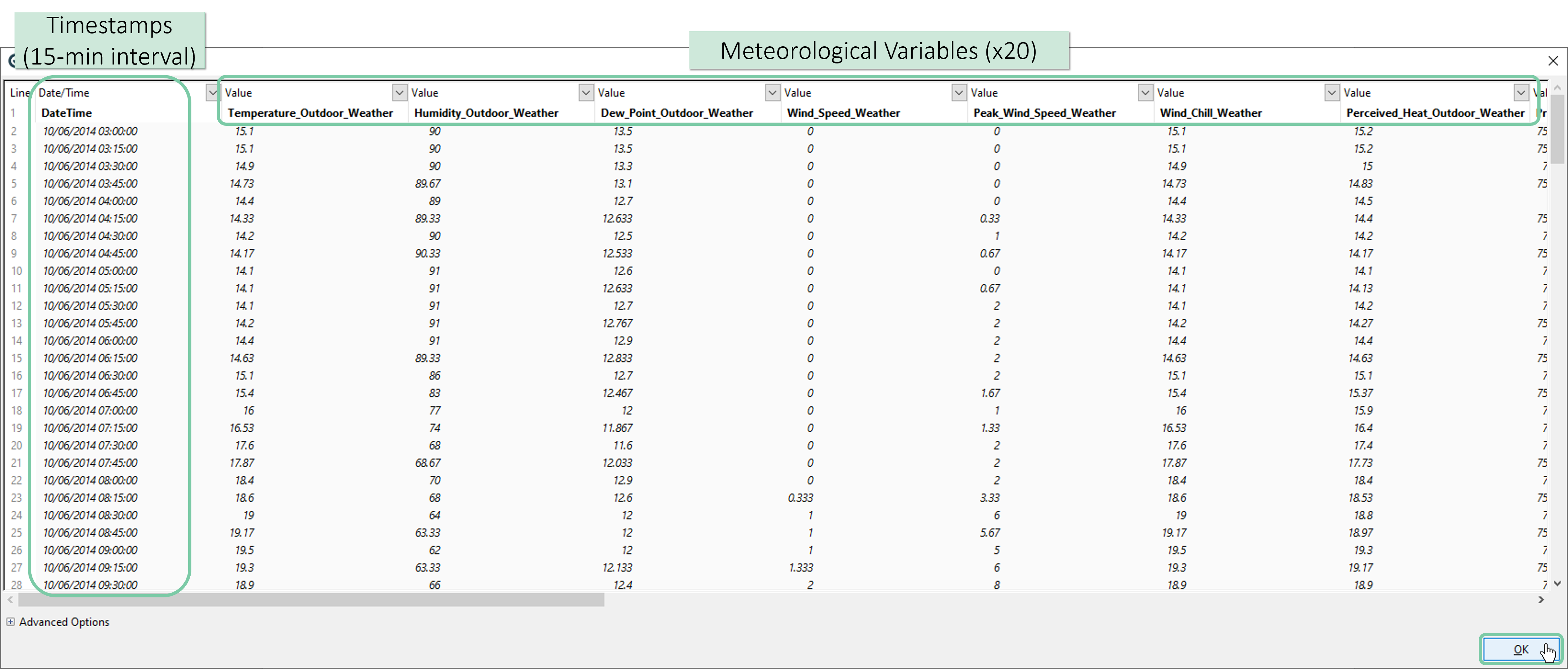
Next, a preview of the data will be shown. This dataset holds 20 meteorological variables measured in 15-minutes intervals from a weather station in the vicinity of the 6 solar power plants (assets). Please have a look at the overview and then click ‘OK’

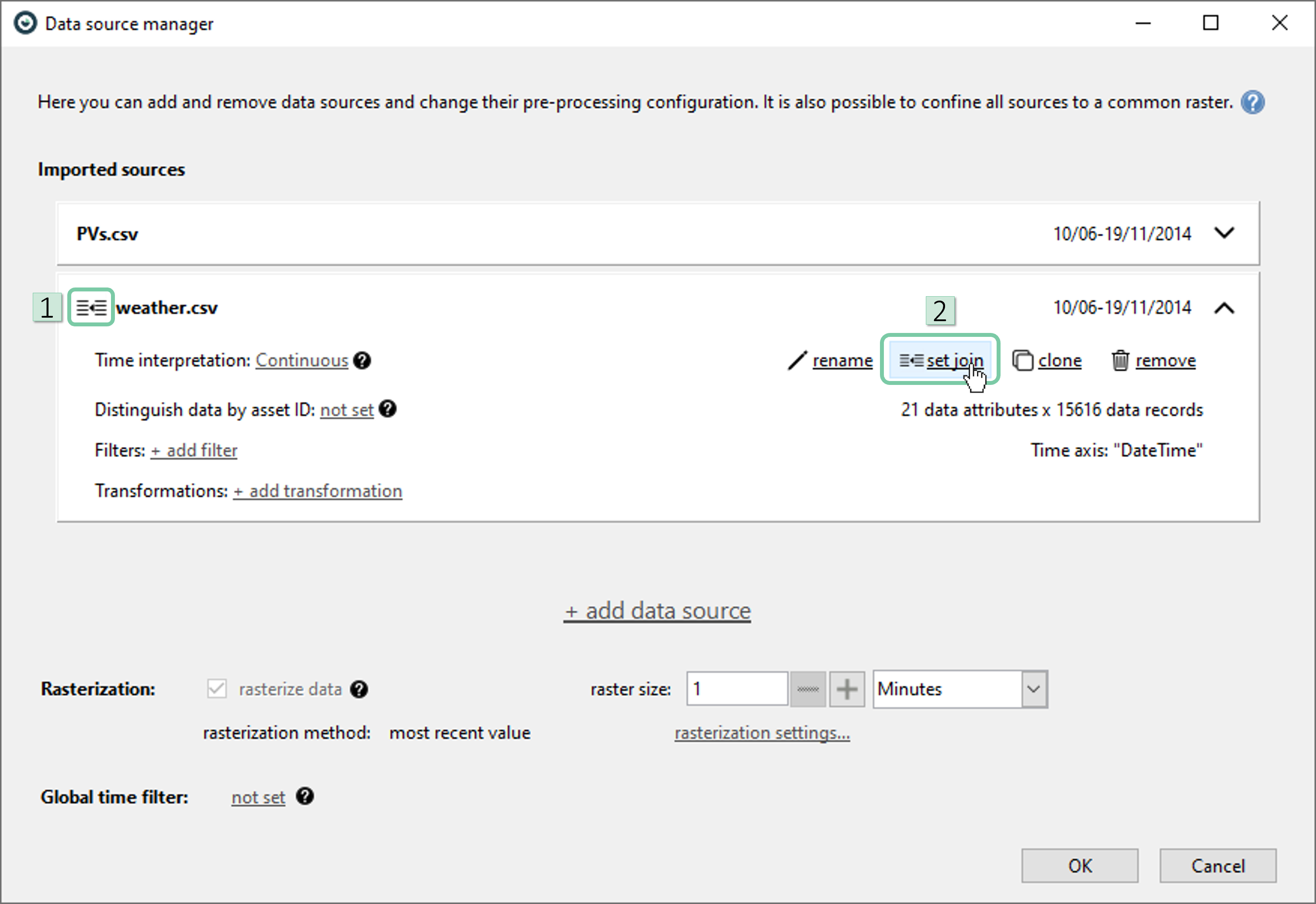
After the import, Data Source Manager will pop-up. Now, you should see two data sources (csv files in this particular case) listed. We would like to merge these data sources in wide format as the aim of this analysis is to find the possible correlations between power generation and weather. Visplore has a clever algorithm that automatically attempts to detect the best merge type (wide or long). In this case, you should see a ‘wide’ merge suggested automatically as shown in the box 1 below. You can always change this selection (not necessary in that case) by clicking ‘set join’.

After wide-merging multiple sources, you will notice that ‘rasterize data’ box is checked automatically, and it is not possible to uncheck it. This is due to Visplore needing a common temporal resolution for merging multiple data sources in wide format. For example, in our case the power data is in 10-minutes resolution and weather data is in 15-minutes resolution. Therefore, a common temporal resolution is needed.

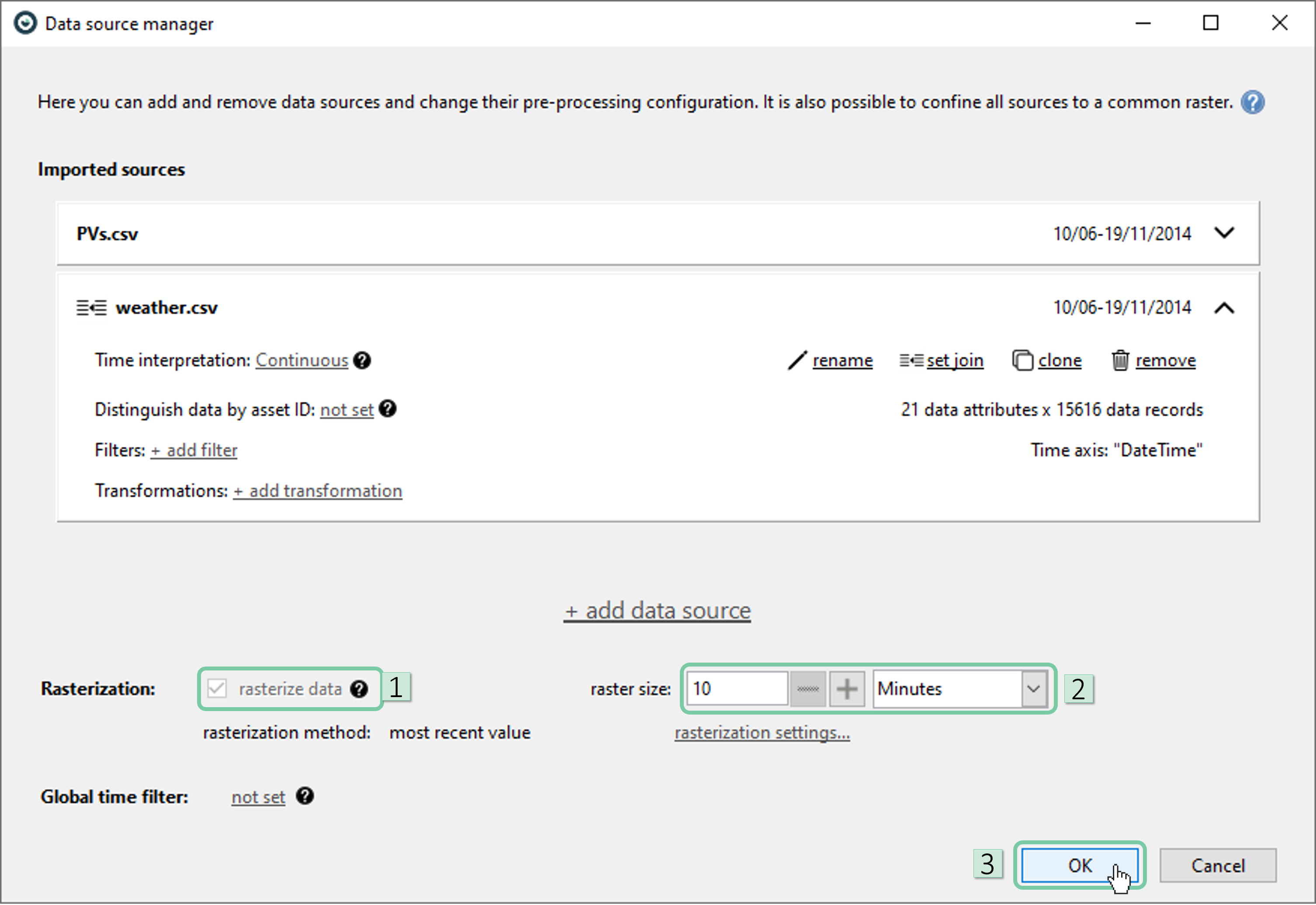
Set the raster size to 10 minutes and click ‘OK’

Please visit one of our other guides, Getting your data in shape, for more on transformations and rasterizations.

Correlating wide-merged data sources

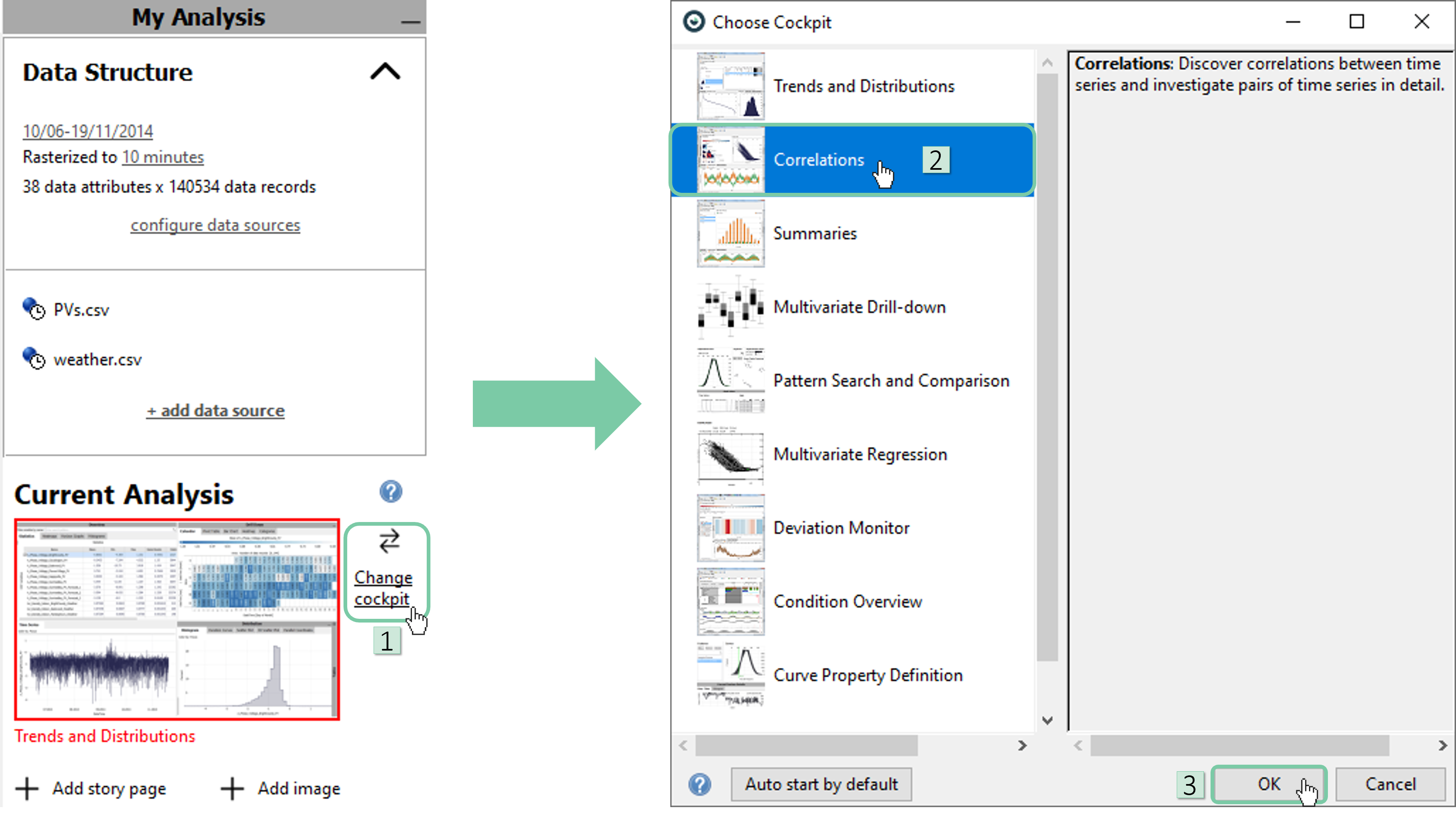
Let’s switch to the correlation cockpit. Click ‘Change cockpit’ in the ‘My Analysis’ pane and select ‘Correlations’ from the cockpit list. Then, click ‘OK’

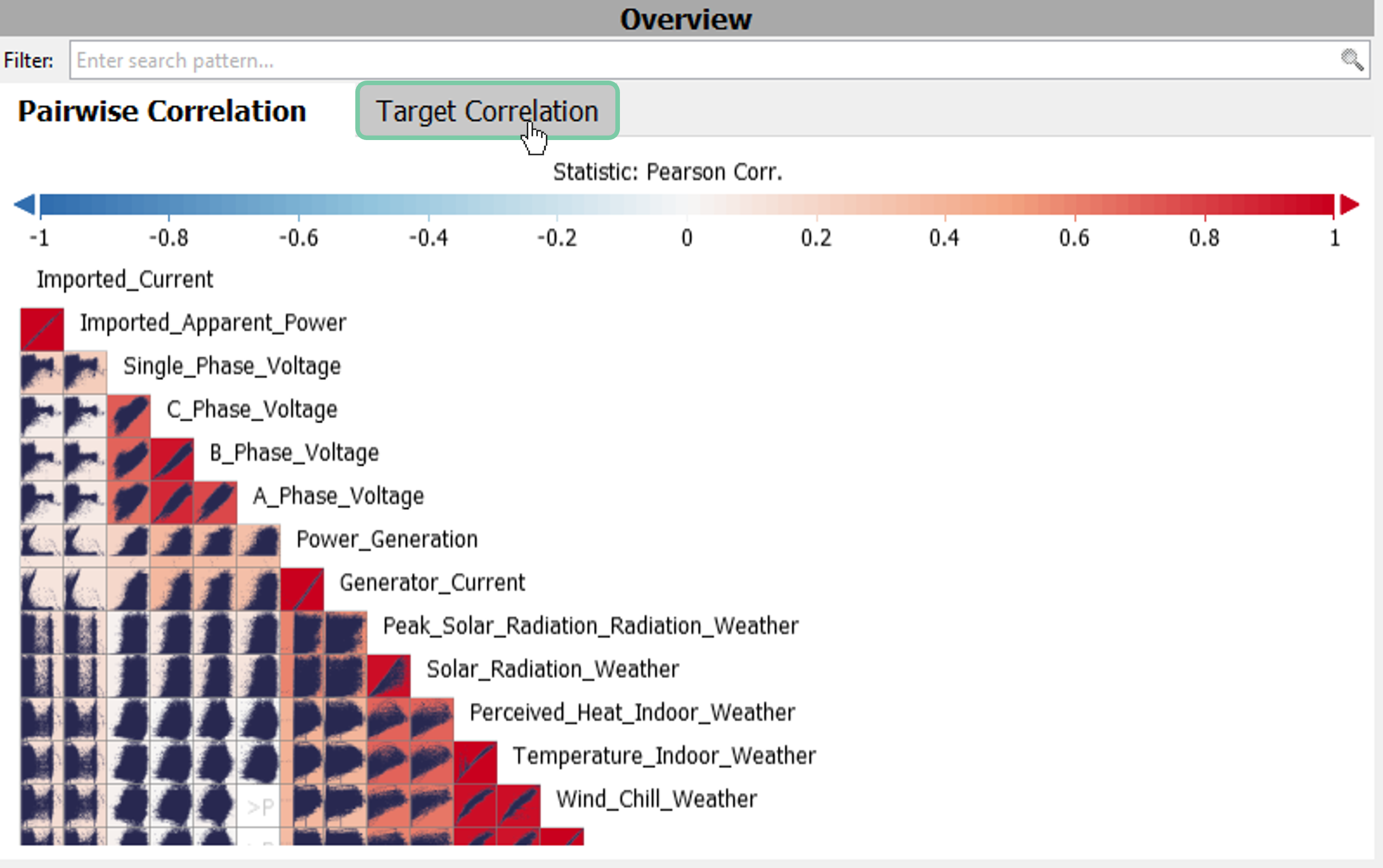
Select ‘Target Correlation’ as shown.

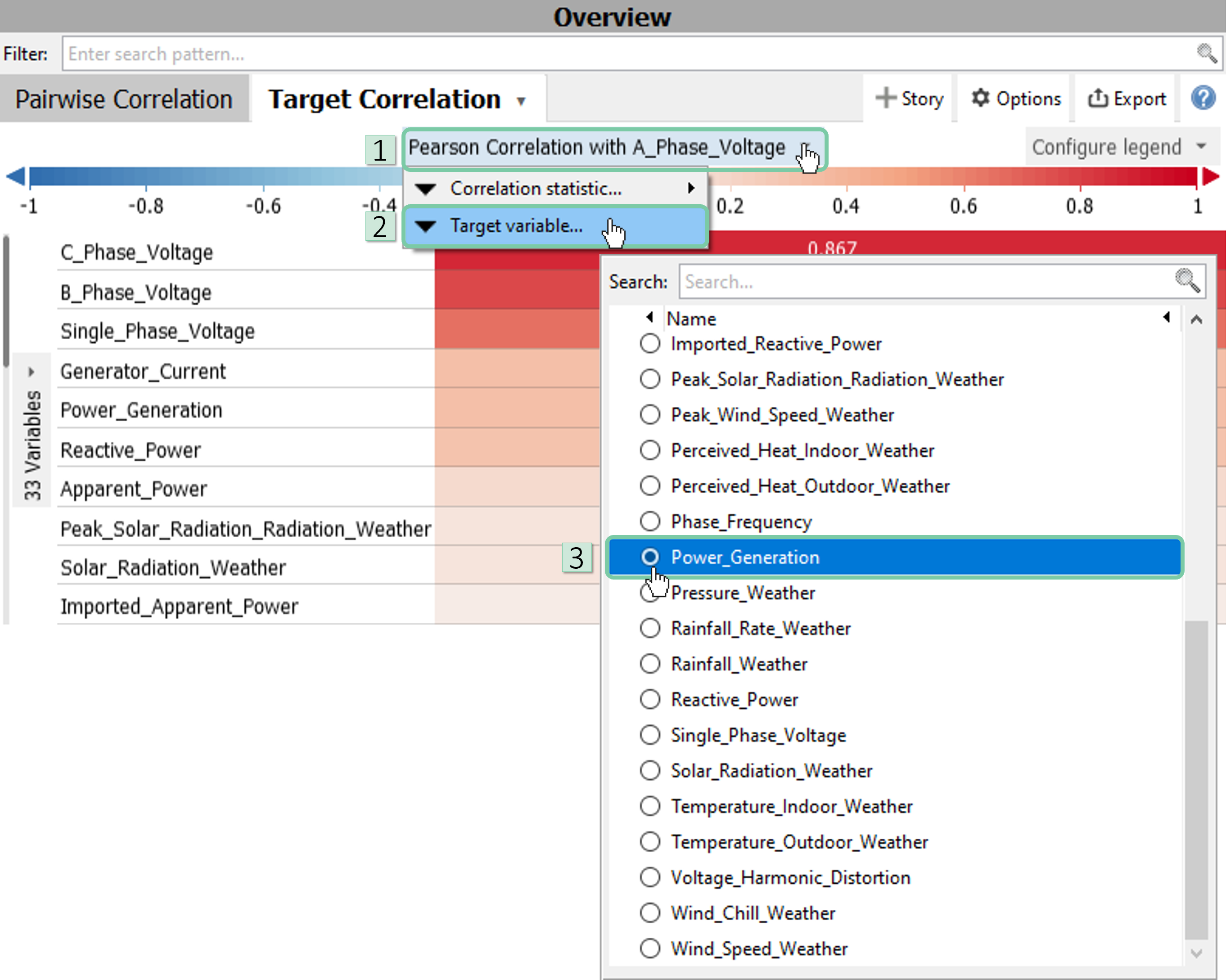
To change the target variable, click on the grey area as shown. Then click ‘Target variable…’ and select ‘Power_Generation’ from the list.

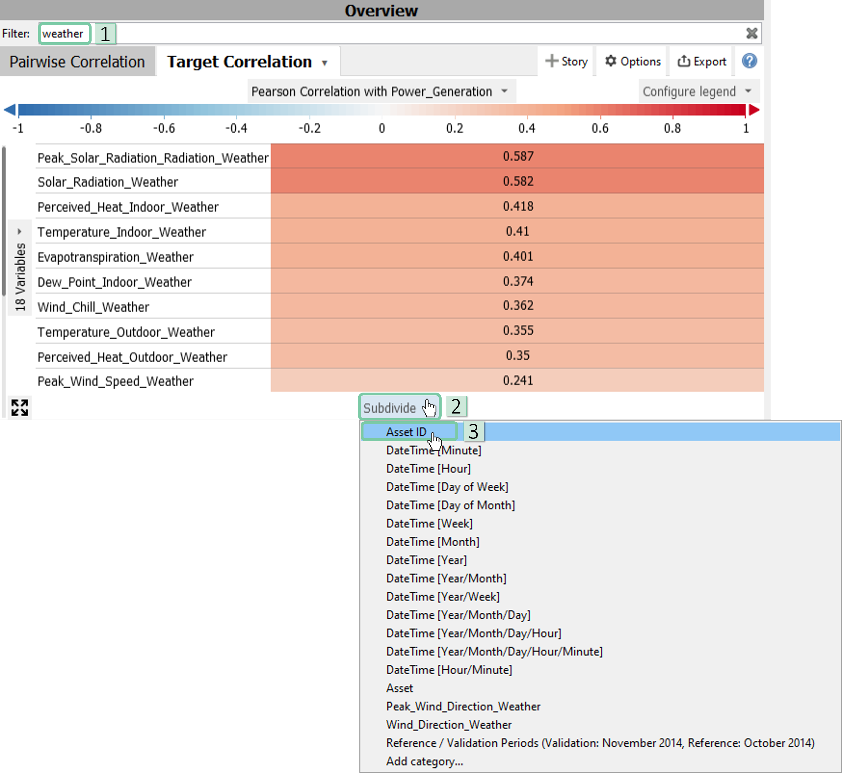
As we want to see the correlation between power generation and weather conditions, filter the variables using the filter bar by writing ‘weather’. Then, subdivide the x-axis using the Asset ID.

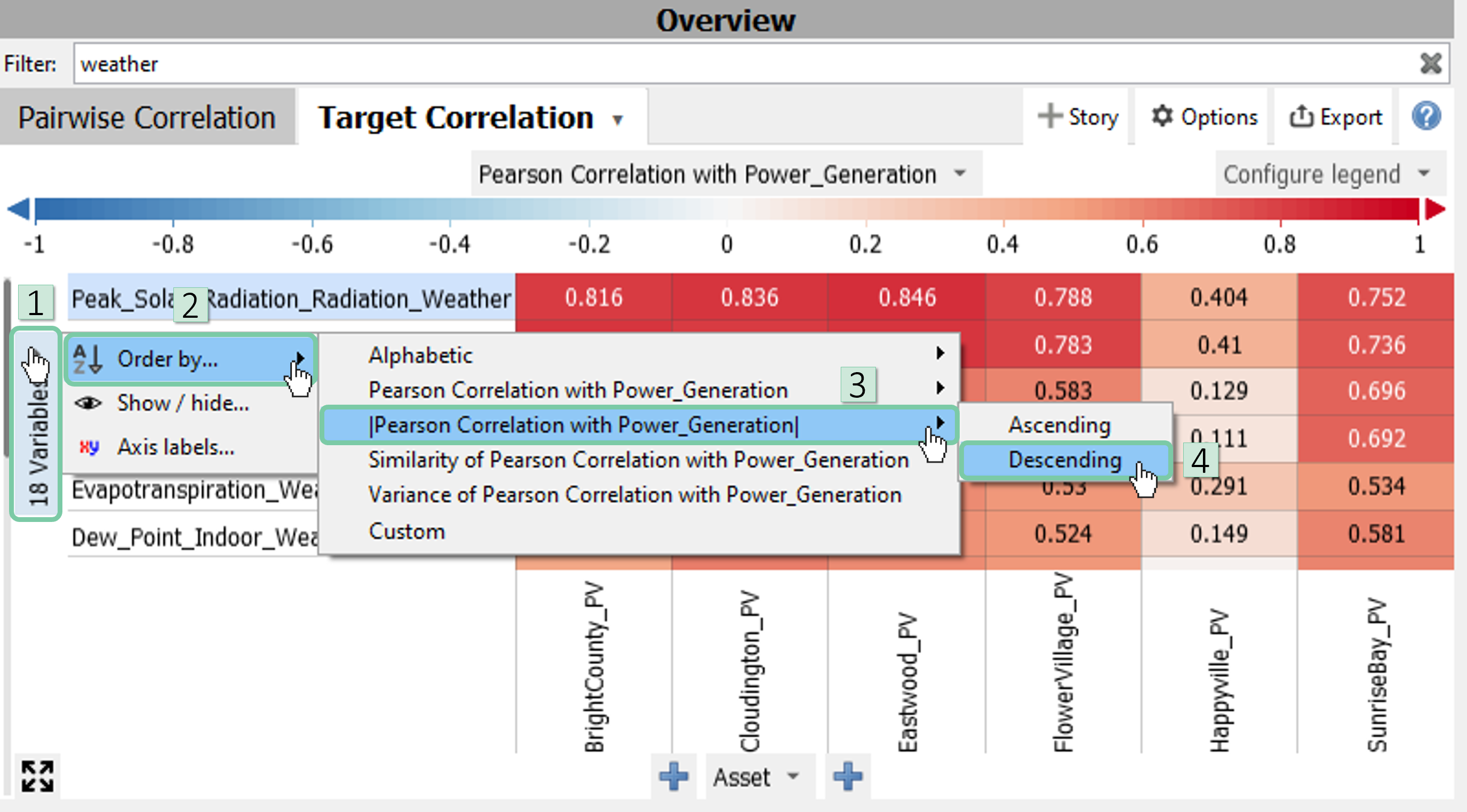
To order variables by the absolute value of their correlation coefficients, click to the grey area on the y-axis where it says ’18 variables’. Then follow the path shown in the image below.

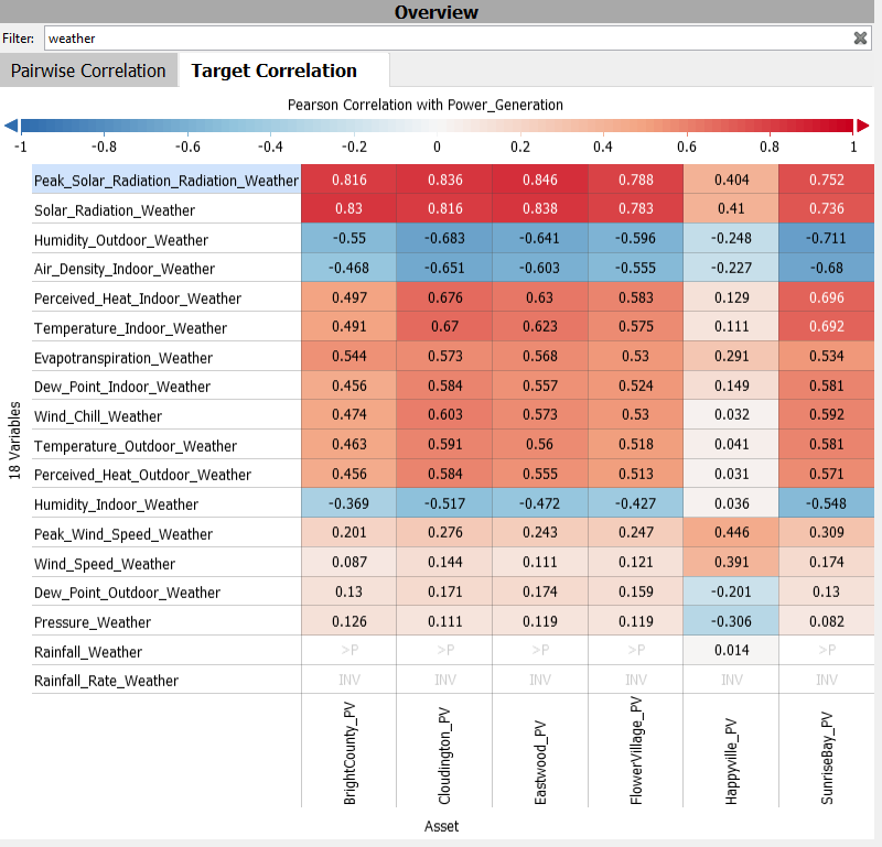
Looking at the correlation matrix, now it is clear that power generation is highly correlated with solar radiation and moderately correlated with humidity, air density and temperature. Also notice that thanks to the asset IDs we have also identified that Happyville differs from other power plants. This is a valuable indicator for engineers to look for the cause behind it.

Long-Merging data sources for comparison

Although wide-merging might be pretty handy for correlation analysis, long-merging is a better option for comparisons of different timespans with similar data structures, i.e. merging a separate file for each month of operation in a manufacturing environment.

Let’s have a look at how long-merge can be utilized in Visplore. In this analysis we would like to compare the power generation in summer versus fall. We will be using the same data source from the previous wide-merge example.

Start a new session and as described in the earlier parts of this guide, load the ‘PVs’ CSV file. This time, accept the automatically detected Asset ID and Variable columns, i.e., do not uncheck the boxes. Proceed until you see the Data Source Manager (DSM) window.

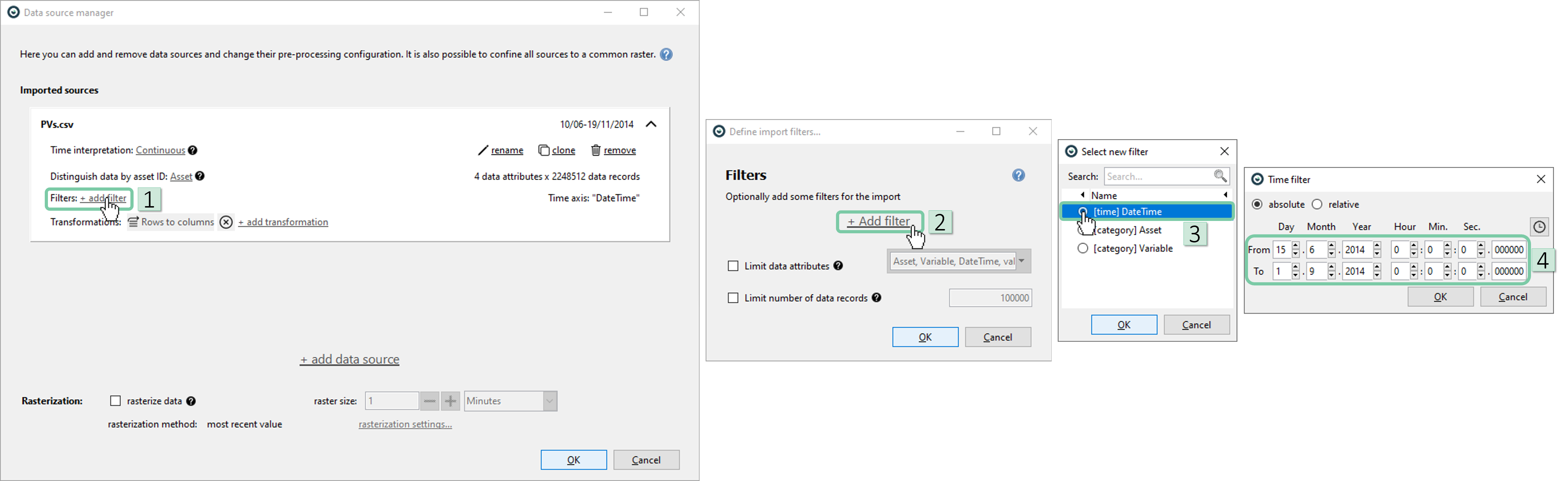
In the DSM window, click ‘add filter’ and follow the below sequence to add a time filter that filters a 2,5 months long timespan in summer from 15.06.2014 to 01.09.2014, Then click ‘OK’ until only the DSM window is left open.

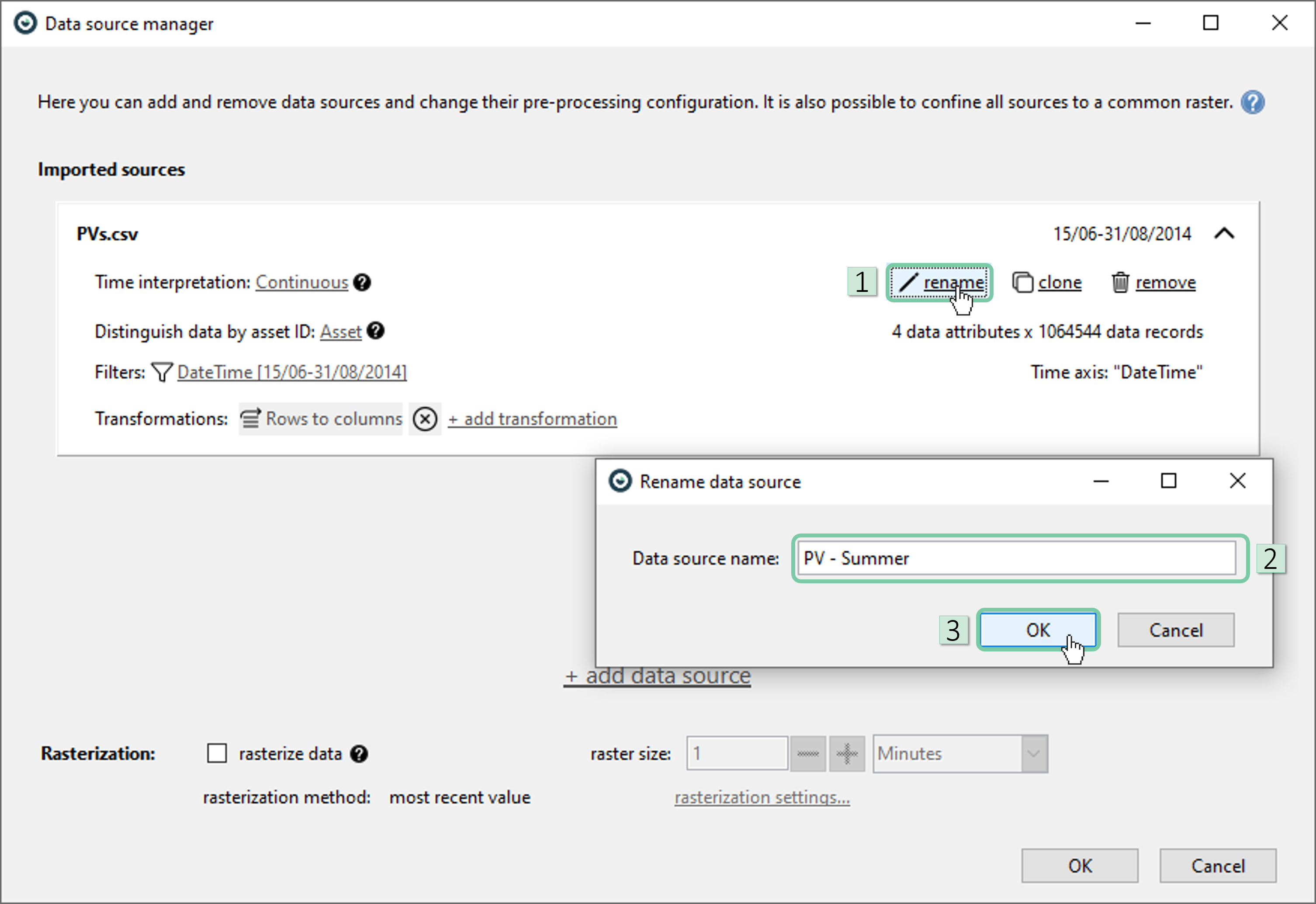
In the DSM window, rename the data source to a more meaningful name that indicates its timespan.

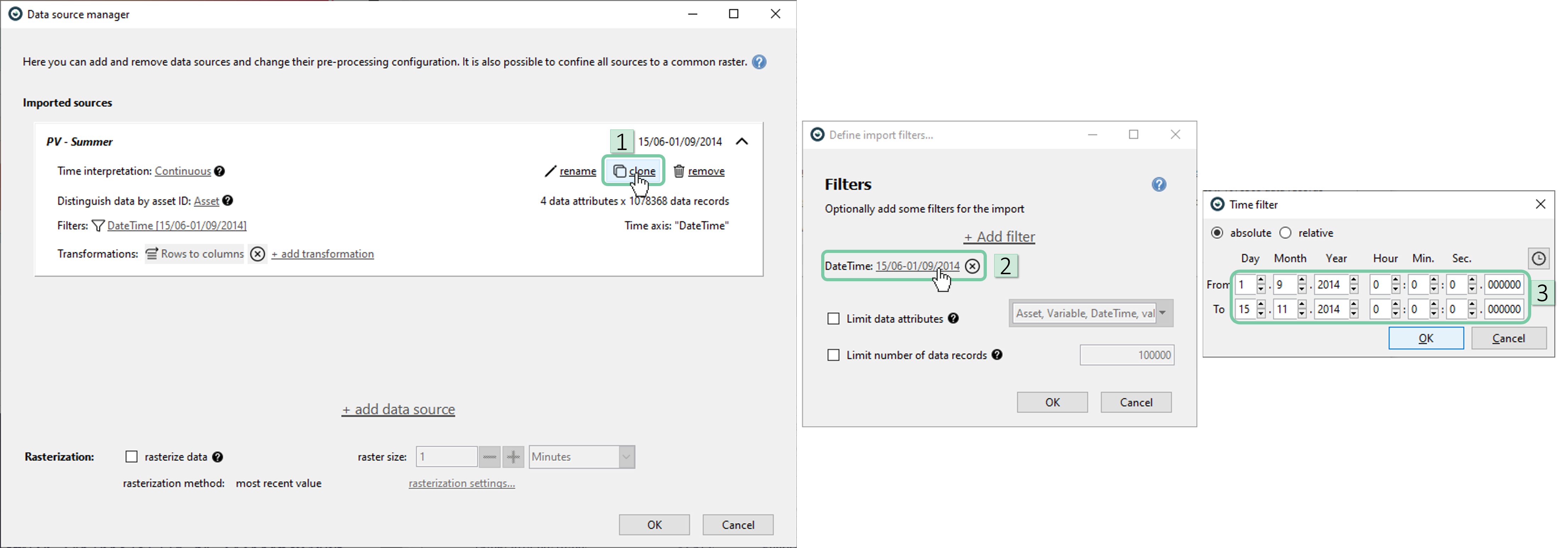
Now, clone this data source and change the timespan to another 2,5 months long timespan in fall from 1.09.2014 to 15.11.2014. Similarly, rename this source to ‘PV – Fall’.

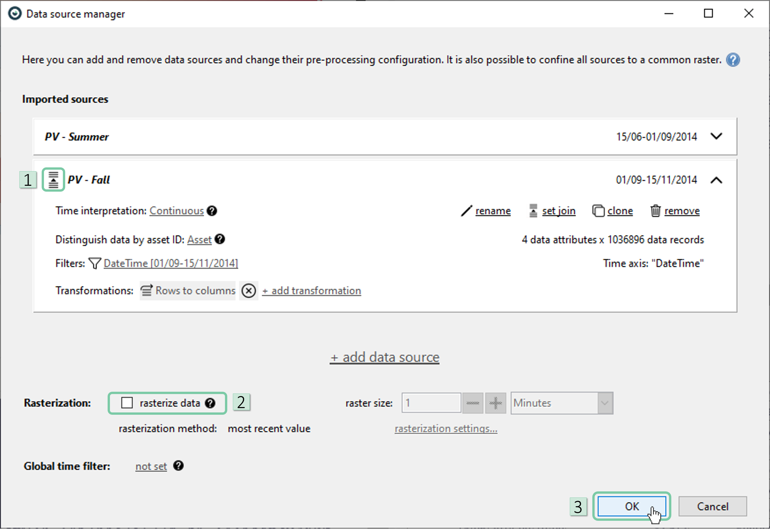
Please note that, this time the algorithm automatically suggests a long merge. Also notice that the rasterization checkbox is not automatically checked, as a long merge does not require it to be checked. Just click ‘OK’ now.

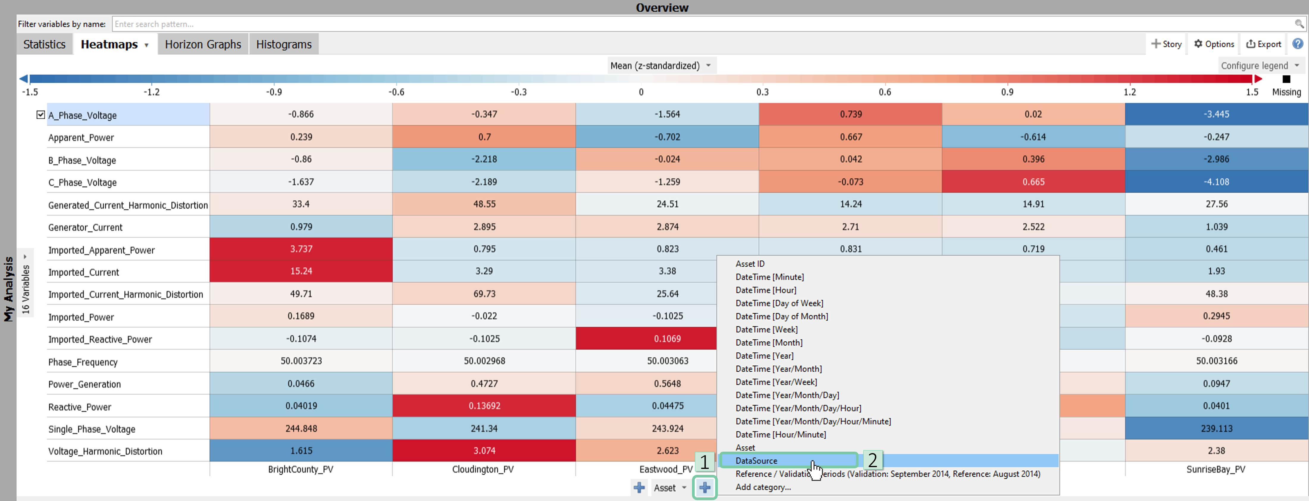
In the Heatmap view, click the ‘+’ icon on left and add ‘DataSource’ ass a partitioner. If you can locate it in the list, click ‘Add category…’ to add it to the list first.

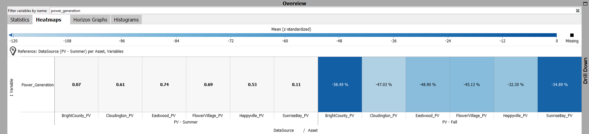
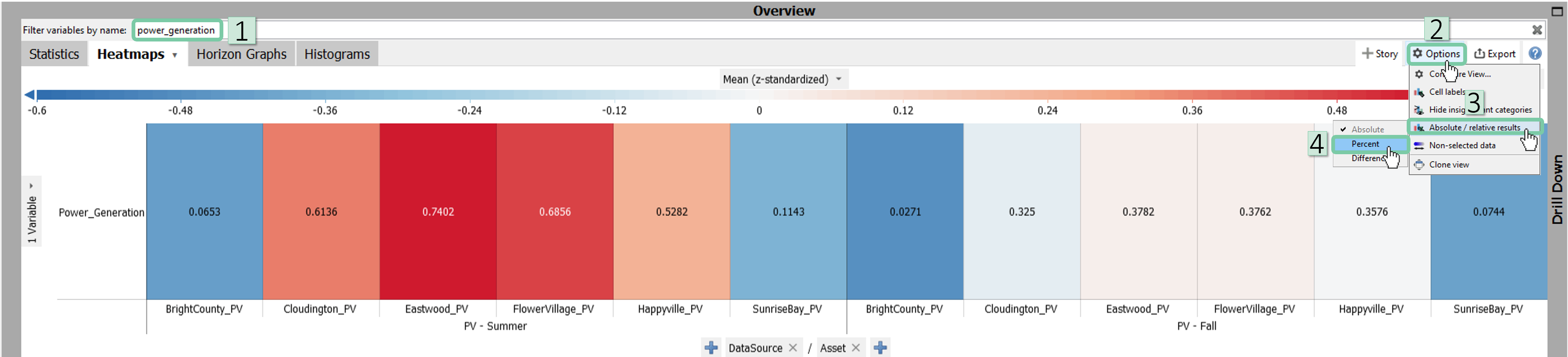
As we aim to compare power generation between summer and fall, write ‘Power_Generation’ into the filter bar. Then, switch to the percentage scale by clicking ‘options’ on top right of the ‘Overview’ window and then following the sequence shown in the below image.

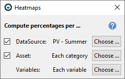
Below dialog will appear. We want to calculate the percentages per asset while taking the summer months’ average as benchmark. For that purpose, adjust the settings as shown below.