Analyzing tables in long format
Data tables in 'long' format are increasingly common for IoT/sensor data and time series databases. 'Long' means that different time series are not (or not only) represented by different columns of the table, but additionally need categories of categorical column(s) to be uniquely identified. A simple example is a 'Device name', 'Location' or other ID in a categorical column, that refers to independent assets. Therefore, with additional assets, such a table becomes 'longer', and not 'wider' as would be the case with wide tables. Timestamps can occur multiple times (once per category), or be very different for each sensor, which is also in contrast to typical wide tables. The image below shows an example of different Wind_turbine_names as asset categories:
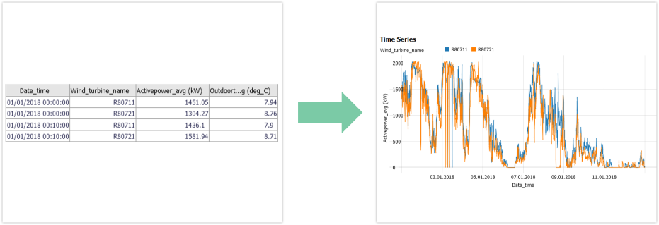
In Visplore, the distinction by assets is not made automatically. This chapter describes, which settings should be set in order to effectively explore and analyze data tables in long format, based on an open Wind Power dataset you can download from here: ENGIE La Haute Borne windfarm dataset (modified, see credits at bottom of page). Some types of analysis will only work for tables in wide format, e.g. computing a correlation coefficient between different assets. Therefore, this chapter also describes the transformation of long to wide tables, which can be achieved in Visplore using Pivot tables.
Settings to work with data in long format
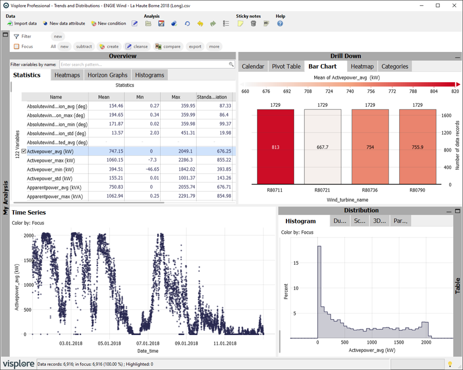
When loading a table in long format in Visplore (e.g. the demo CSV from above), Visplore will treat all 'assets' as part of the same variable (e.g. a mean value across all measurements, regarding which wind turbine they are from). In most cases, this is not desired, but assets should be treated independently. Look at the image below. The timeline holds measurements from all four turbines (the 'asset categories'). Also, the timeline is showing discrete points instead of connected lines by default, because each timestamp occurs multiple times (once per wind turbine), and therefore is not assumed to be a continuous time series.
You need to make a couple of configurations in Visplore, to work with such datasets in long format appropriately.
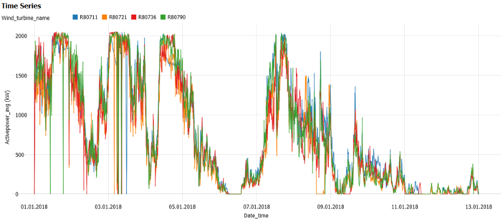
First, we recommend you distinguish assets by color, and make the display of the Time Series view continuous.

With one continuous line per asset category, now it is easy to distinguish the values of the 4 wind turbines. You can also plot the variables of each wind turbine separately, but it requires further settings:
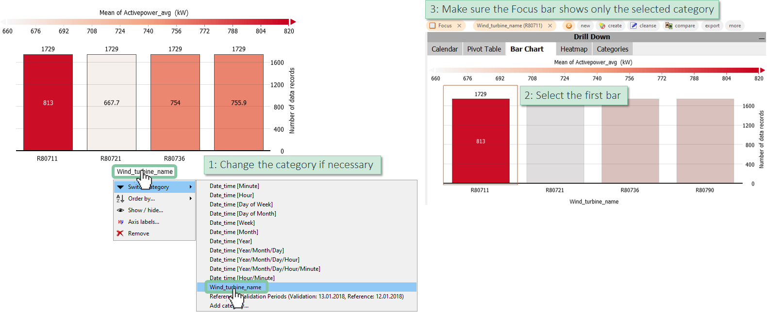
As next step, we suggest to adjust either the Bar Chart or the Pivot Table tab to show the different wind turbines - in order to focus on specific assets at time. In this example, we are making the necessary settings in the Bar Chart tab, which you find in the "Drill Down" block in the top right corner of Visplore.
Make sure, the "Wind_turbine_name" category is displayed as the main category of the bar chart (see here to recap details on how to do this).
Select (=click) one bar to put one of the wind turbines in focus as shown in the image on the right. Before this step, make sure the Focus bar is empty.
The last step is to hide non-selected data in the Time Series view, so you won't see the data that are not in focus (= all non-selected turbines).

Great! You have made the settings needed to work with a dataset in long format. If you want, you can save the configurations as a .visplore template, which you can apply to new data of the same structure next month again.
Basic workflow at this point:- Click on a bar of an asset (e.g. Wind turbine) in the Bar Chart to display only that asset in Time Series and other views.
- Hold CTRL while clicking a bar for selecting multiple assets.
- Use the 'Statistics' in the 'Overview' block in the top left to select, which variables are shown in the Time Series for each asset.
- To distinguish multiple variables by color instead of multiple assets, click the 'x' in the color legend in the Time Series plot. If you want to get back to distinguishing assets by color, repeat the 'color by' setting from the beginning of this section.
- If you have multiple categorical columns that make an asset unique (e.g. 'device ID' and 'location'), we recommend using a filter to consider only one 'location' at time, then use the rest of this chapter to analyze assets per 'device ID'. Or, if you want to compare locations, do it the other way around, and put 'device ID' in the filter.
- To see the correlation between the sensors of the same asset in a Scatter Plot, you need to repeat the configuration steps of this section for the "Scatter Plot". So, configure the coloring of the scatter plot, select an asset category in the Bar Chart or Pivot Table and hide the 'Non-selected data' in the Scatter Plot, just the same way as was shown for the Time Series plot, before in this chapter.

Advanced workflow tips for datasets in long format:
- For data labeling and defining conditions on individual assets, select the asset category first by choosing a bar in the Bar Chart or a row in the Pivot Table. Then hit the
 button in the focus bar, then select the data points to label. Only label a single selection (e.g. time period) at once in this case and avoid using the '+' (CTRL) key for multi-selection, because concatenated selections may not be referring to a single asset at a time. If you want to use multi-selection for your labeling workflow, make sure to filter for a single asset first.
 - For pattern searching within a single asset, define a filter on that asset first, then search the pattern.
- For computing a Pearson correlation between different assets, you need to transform the data to wide format first.
- To properly use the Multivariate Regression cockpit, you also need to transform the data to wide format first.
Transforming long tables to wide tables in Visplore
It is possible to transform the dataset to wide format directly in Visplore. You can use the Pivot table, to build the desired table in Wide format directly in Visplore (rastered timestamps as rows, assets/variables as columns). Do this as follows:
If you have a focus or filter defined, clear them for now (press the small "x" symbols next to the words "Filter" and "Focus" at the top of Visplore 
 )
)
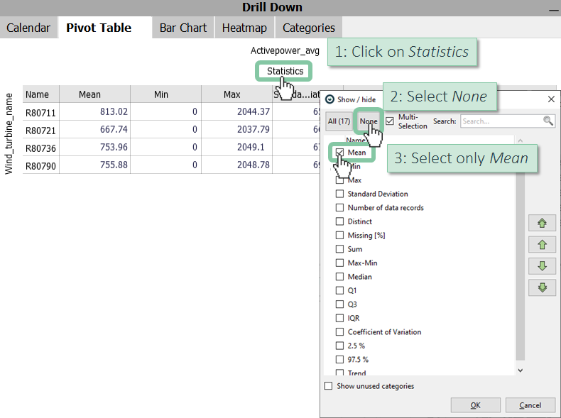
Open the Pivot Table (in the "Drill Down" section of Visplore, in the top right) and hide every statistics except the 'Mean' value.
You need to change the category on the Y-axis to see the mean values in a minute raster for the whole period. Note: this will aggregate all samples of the same minute to one row in the Pivot Table. As we only have a 10-minute resolution in our data, there will only be 10-minute timestamps shown, despite us allowing up to minute resolution.
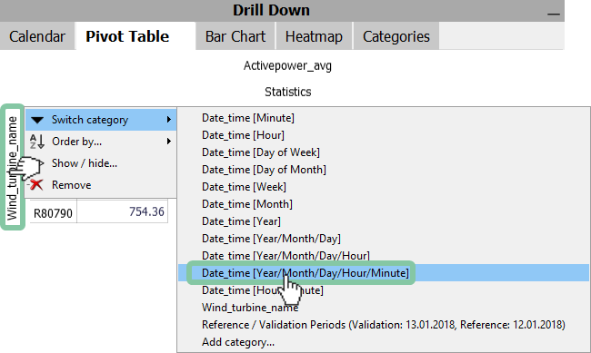
Note: If you want hourly mean values, choose the "Year/Month/Day/Hour" category instead.
Now you need to subdivide the 'Mean' value by the Wind_turbine_name category so every turbine is displayed.
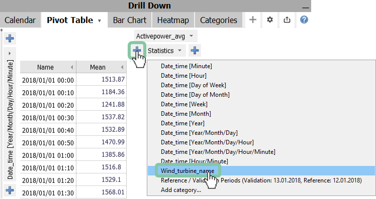
Note: In case you have more than one asset category you need to use multiple subdivisions.
The last step before exporting to wide format is the selection of the sensor variables we want to keep in our wide table. Do this by using the checkmarks in the 'Statistics' plot. If you want to select all of them, an easy way to do this is: [1] select the first variable (Absolutewinddirection_avg) in the Statistics view, [2] scroll down to the last variable, [3] hold down the 'Shift' key on your keyboard, [4] select the last variable (Windspeed_std).

Now the Pivot Table is set, so you can export it and load it in a new Visplore instance.
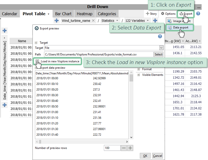
Great! Now a new Visplore instance is loaded with the dataset in wide format. Using the wide format, you can compute a Pearson correlation between the different assets and use the Multivariate Regression cockpit.
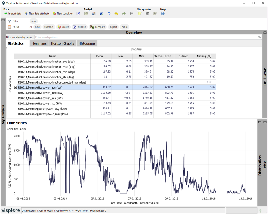
ENGIE La Haute Borne windfarm dataset is used for screenshots.
Source of Dataset (in its original form): https://opendata-renewables.engie.com/
License: Open License version 2.0 published by Etalab: https://www.etalab.gouv.fr/wp-content/uploads/2018/11/open-licence.pdf
Dataset was modified (e.g. columns renamed) for easier communication of Visplore USPs. Download the modified version, to follow our demo examples, from here.
